Chapter 2 Shiny

Watch this video before beginning

Shiny is a modern programming miracle and it helps to make R one of the most competitive languages for communicating insights from data. Shiny is developed by RStudio and it is described as “A web application framework for R”. Unlike web application frameworks in many other languages the time it takes to write a beautiful, functional, and mobile-ready Shiny application is truly minimal, which makes it ideal for rapid prototyping and easy deployment. The folks at RStudio have the following pitch: “Turn your analyses into interactive web applications No HTML, CSS, or JavaScript knowledge required”. This statement is mostly true, though a little HTML knowledge is useful for understanding some of the concepts. If you’re interested in learning more about HTML, CSS, and Javascript we recommend any one of the following resources:

We’ll proceed as if your HTML knowledge is very basic and no more advanced than understanding heading levels or fonts.

2.1 Installing Shiny

First, make sure you have the latest release of R installed. If on Windows, make sure that you have Rtools installed. Then, you can install shiny with

install.packages("shiny")
libray(shiny)

2.2 Your First Shiny App

Let’s build our first app. Like many projects in this book, we’ll start with a simple example app. First create a new directory where you can store all of the files associated with your app. I like to organize my shiny app into two separate files: ui.R which contains all of the user interface elements of the app, and server.R which contains the logic of the app, including code for loading and handling data. You can find the code for each of these files below:

App 1: ui.R

library(shiny)

fluidPage(
  titlePanel("Data science FTW!"),
  sidebarLayout(
    sidebarPanel(
      h3("Sidebar Text")
    ),
    mainPanel(
      h3("Main Panel Text")
    )
  )
)

App 1: server.R

library(shiny)

function(input, output){
  
}

This app is extremely minimal, it’s just meant to get you familair with the syntax of shiny apps including the nested nature of the user interface elements. Create these two files inside of your new directory, then change your current working directory to that folder using setwd(). After loading shiny with library(shiny) enter runApp() into the R console to start the app. Alternatively you can provide the path to the directory containing the ui.R and server.R files as an argument to runApp(). You app should look something like this:

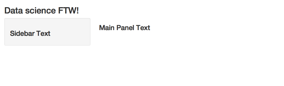
Your First Shiny App

Let’s walk through the code in ui.R. The fluidPage() function specifies a type of user interface for Shiny to display. Fluid pages try to intelligently rearrange themselves depending on the size of the screen that’s displaying the app which makes this layout look better on mobile devices. Instead of a fluidPage() you could use a fixedPage() which will not resize your app. The titlePanel() function defines a title on the top of the page and the sidebarLayout() function defines the layout for everything below the title panel. The sidebarLayout() splits the page into a sidebar and a main part of the page, which are then specified with the sidebarPanel() function and the mainPanel() function respectively. Inside the sidebarPanel() and the mainPanel() I put an h3() heading, which just displays some text and is the same as specifying an <h3> tag in HTML.

The ui.R simply defines the layout of the page. If you run the code in ui.R on it’s own you can see that a standard set of HTML tags are returned:

<div class="container-fluid">
  <h2>Data science FTW!</h2>
  <div class="row">
    <div class="col-sm-4">
      <form class="well">
        <h3>Sidebar Text</h3>
      </form>
    </div>
    <div class="col-sm-8">
      <h3>Main Panel Text</h3>
    </div>
  </div>
</div>

All Shiny is doing is piecing together some HTML!

2.3 More UI Elements

Let’s take a look at another simple app with a slighly more complex UI:

App 2: ui.R

library(shiny)

fluidPage(
  titlePanel("HTML Tags"),
  sidebarLayout(
    sidebarPanel(
      h1("H1 Text"),
      h3("H3 Text"),
      em("Emphasized Text")
    ),
    mainPanel(
      h3("Main Panel Text"),
      code("Some Code!")
    )
  )
)

App 2: server.R

library(shiny)

function(input, output){
  
}

The code above will produce an app like this:

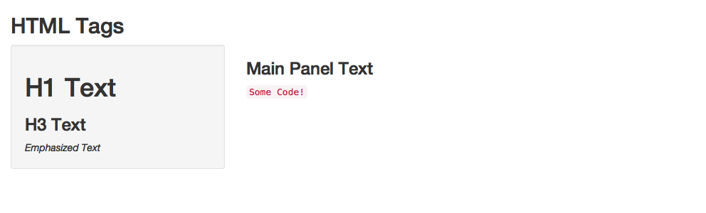
A Second Shiny App

In this example we’ve added a few UI elements and you can see how they are rendered in the app. The h1() and h3() functions specify headers, the em() function italicizes text, and the code() function renders the text with a monospaced font to make it look like computer code. You can find a listing of all of the different UI text tags that are availible by typing ?builder into the R console.

2.4 Inputs and Outputs

Now that you know the basics of the Shiny user interface you can start to learn how to make your Shiny apps do something useful! The most important feature of a web application is that a user can provide input through interacting with your app, and then you can show the user outputs that respond to those inputs. Let’s start with the following simple Shiny app:

App 3: ui.R

library(shiny)

fluidPage(
  titlePanel("Slider App"),
  sidebarLayout(
    sidebarPanel(
      h1("Move the Slider!"),
      sliderInput("slider1", "Slide Me!", 0, 100, 0)
    ),
    mainPanel(
      h3("Slider Value:"),
      textOutput("text")
    )
  )
)

App 3: server.R

library(shiny)

function(input, output){
  output$text <- renderText(input$slider1)
}

The code above will produce an app that looks like this:

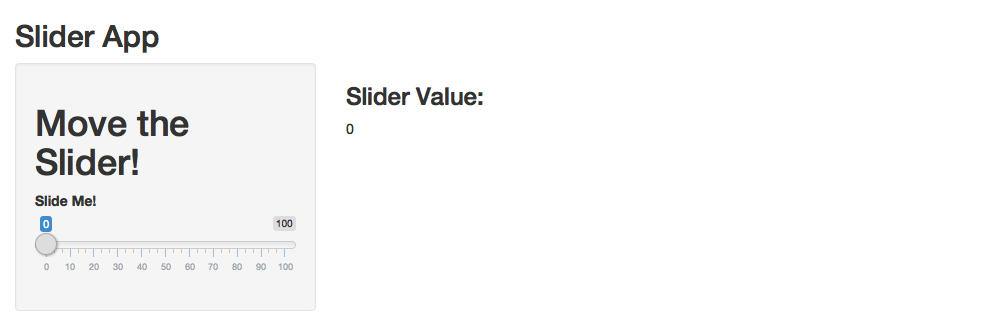
A Simple Slider

A screenshot of this app doesn’t do it justice, make sure you run this app on your own computer! You can do this easily by entering the following into your R console:

shiny::runGitHub("seankross/developing-data-products", subdir = "assets/shinyapps/app3/")

Try sliding the slider back and forth. The number displayed on the page should change to reflect the value of the slider. In ui.R the only new function is sliderInput() which defines the slider user interface element on the page. This function takes several arguments including a unique identifier for this slider ("slider1" in this case), text to be displayed above the slider, and finally minimum, maximum, and inital values for the slider.

The second new function in the UI is textOutput(). This function renders text that is computed in server.R. The only argument passed to this function is a string with the ID of the text which is specified in server.R. We’ll designate a simple ID called "text" which we’ll use later in server.R.

This app is the first one I’ve showed that has something notable going on in server.R. The server.R file must return a function, so for simple apps it’s appropriate to define a anonymous function like we’ve done in this example. This function must have arguments named input and output. You should think of the values of these arguments inside of the server function as a list() which each have named elements that you can query (in the case of input) and assign values to (in the case of output). In this example we’re retrieving the value of the slider from input according to the identifier we assigned to it in ui.R ("slider1"). The expression input$slider1 evaluates to the current value of the slider. We then wrap that expression with the renderText() function which renders a value so it can be printed as text in a Shiny app. The rendered value is then stored in the output list in the text element. The app’s UI is then able to retrieve this value since we specified the text ID in ui.R, and the value of the slider is thus displayed on the screen.

If you understand how the app describe above is working, then you understand basic input and output in Shiny! On the server side of a Shiny app, you’re often writing code that takes inputs from the UI, does some computation, and you must render the result of that computation in order to show it to the user. Usually you can accomplish this with the render family of functions included in Shiny. In the next app we’ll take a look at showing a plot to the user based on some inputs, eventually using the renderPlot() function.

App 4: ui.R

library(shiny)

fluidPage(
  titlePanel("Plot Random Numbers"),
  
  sidebarLayout(
    sidebarPanel(
      numericInput("num_points", "How Many Random Numbers Should be Plotted?", 
                   value = 1000, min = 1, max = 1000, step = 1),
      sliderInput("sliderX", "Pick Minimum and Maximum X Values",
                  -100, 100, value = c(-50, 50)),
      sliderInput("sliderY", "Pick Minimum and Maximum Y Values",
                  -100, 100, value = c(-50, 50)),
      checkboxInput("show_xlab", "Show/Hide X Axis Label", value = TRUE),
      checkboxInput("show_ylab", "Show/Hide Y Axis Label", value = TRUE),
      checkboxInput("show_title", "Show/Hide Title")
    ),
    
    mainPanel(
      h3("Graph of Random Points"),
      plotOutput("plot1")
    )
  )
)

App 4: server.R

library(shiny)

function(input, output) {
  output$plot1 <- renderPlot({
    set.seed(2016-12-13)
    
    dataX <- runif(input$num_points, input$sliderX[1], input$sliderX[2])
    dataY <- runif(input$num_points, input$sliderY[1], input$sliderY[2])
    
    xlab <- ifelse(input$show_xlab, "X Axis", "")
    ylab <- ifelse(input$show_ylab, "Y Axis", "")
    main <- ifelse(input$show_title, "Title", "")
    
    plot(dataX, dataY, xlab = xlab, ylab = ylab, main = main,
         xlim = c(-100, 100), ylim = c(-100, 100))
  })
}

The code above will produce an app that looks like this:

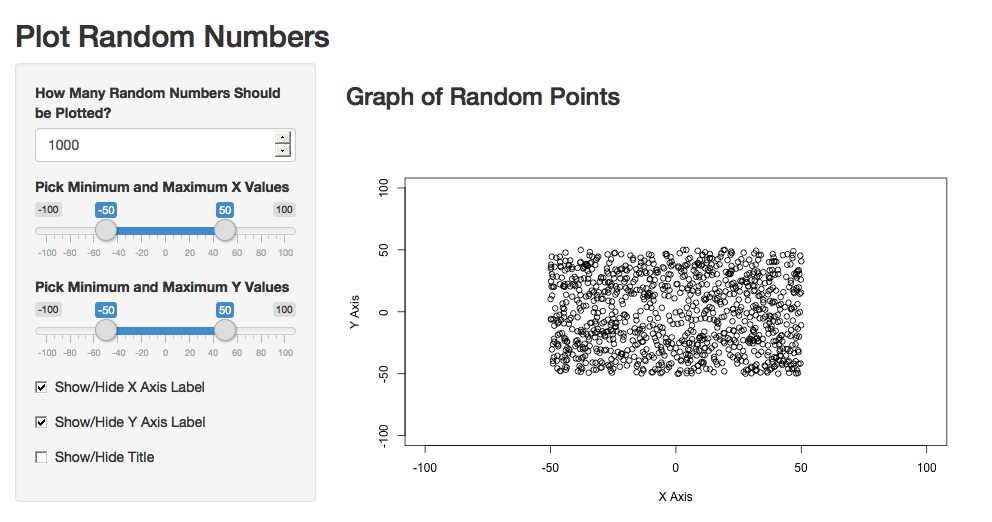
Plot Random Points

You can run the app locally with this line of code:

shiny::runGitHub("seankross/developing-data-products", subdir = "assets/shinyapps/app4/")

This app has more code than any of the apps we’ve built before, but it’s just an extension of the same ideas we’ve been talking about. In ui.R there are a few new functions. The numericInput() function allows users to type in a number into a text box. You’ve already seen the sliderInput() function, but in this case there are two inital values, which allows the user to select a range of values on a slider between a minimum and maximum value. Next there’s the checkboxInput() function which creates a checkbox on the page that the user can toggle. Finally the plotOutput() function displays a plot that is rendered in server.R.

All of the action in this server.R file takes place within an expression passed to renderPlot() since a plot is the only output of this app. The number of random numbers to generate is retrieved from input$num_points and each slider returns a numeric vector of length two, with the first element as the leftmost slider value and the second element as the rightmost slider value. The axis title is toggled on and off by input$show_title which is TRUE if the checkbox is checked and FALSE otherwise. The same principle applies to the axis labels. Finally the plot is constructed with a regular plot() function using UI inputs as parameters.

2.5 Dynamic UI

You might want to change how the user interface of your Shiny app is displayed depending on other UI inputs in your app. This is a common pattern seen in online forms, where your choice in an early part of a form narrows the potential choices in later parts of the form. Here’s a small app that illustrates how to dynamically change the UI in Shiny:

App 5: ui.R

library(shiny)

fluidPage(
  titlePanel("Dynamic UI"),
  
  sidebarLayout(
    sidebarPanel(
      selectInput("country", "Which Country do you live in?", 
                  choices = c("USA", "Canada")),
      uiOutput("region")
    ),
    
    mainPanel(
      textOutput("message")
    )
  )
)

App 5: server.R

library(shiny)
library(minimap)

function(input, output) {
  output$region <- renderUI({
    if(input$country == "USA"){
      selectInput("state", "Which state do you live in?", choices = usa_abb)
    } else {
      selectInput("pt", "Which province or territory do you live in?", choices = canada_abb)
    }
  })
  
  output$message <- renderText({
    if(input$country == "USA"){
      paste0("You live in the USA in the state of ", input$state, ".")
    } else {
      paste0("You live in Canada in the province or territory of ", input$pt, ".")
    }
    
  })
}

The code above will produce an app that looks like this:

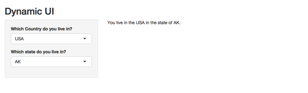
Choose a Region

You can run this app locally like so:

shiny::runGitHub("seankross/developing-data-products", subdir = "assets/shinyapps/app5/")

The ui.R in this app contains elements we’ve seen before except for the uiOutput() function. This function displays UI which is computed inside of server.R! Inside of server.R take a look at the renderUI() function, which contains code you would normally see inside of ui.R. The if statement determines which selectInput() is displayed, either the states of the USA, or the provinces and territories of Canada. Dynamic manipulation the UI can be a powerful tool for controlling the use and flow of your app.

2.6 Reactivity

App 6: ui.R

library(shiny)

fluidPage(
  titlePanel("Predict Horsepower from MPG"),
  
  sidebarLayout(
    sidebarPanel(
      sliderInput("sliderMPG", "What is the MPG of the car?", 10, 35, value = 20),
      checkboxInput("showModel1", "Show/Hide Model 1", value = TRUE),
      checkboxInput("showModel2", "Show/Hide Model 2", value = TRUE)
    ),
    
    mainPanel(
      plotOutput("plot1"),
      h3("Predicted Horsepower from Model 1:"),
      textOutput("pred1"),
      h3("Predicted Horsepower from Model 2:"),
      textOutput("pred2")
    )
  )
)

App 6: server.R

library(shiny)

function(input, output) {
  # Create Spline
  mtcars$mpgsp <- ifelse(mtcars$mpg - 20 > 0, mtcars$mpg - 20, 0)
  
  # Fit Models
  model1 <- lm(hp ~ mpg, data = mtcars)
  model2 <- lm(hp ~ mpgsp + mpg, data = mtcars)
  
  model1pred <- reactive({
    mpgInput <- input$sliderMPG
    predict(model1, newdata = data.frame(mpg = mpgInput))
  })
  
  model2pred <- reactive({
    mpgInput <- input$sliderMPG
    predict(model2, newdata = 
              data.frame(mpg = mpgInput,
                         mpgsp = ifelse(mpgInput - 20 > 0,
                                        mpgInput - 20, 0)))
  })
  
  output$plot1 <- renderPlot({
    mpgInput <- input$sliderMPG
    
    plot(mtcars$mpg, mtcars$hp, xlab = "Miles Per Gallon", 
         ylab = "Horsepower", bty = "n", pch = 16,
         xlim = c(10, 35), ylim = c(50, 350))
    if(input$showModel1){
      abline(model1, col = "red", lwd = 2)
    }
    if(input$showModel2){
      model2lines <- predict(model2, newdata = data.frame(
        mpg = 10:35, mpgsp = ifelse(10:35 - 20 > 0, 10:35 - 20, 0)
      ))
      lines(10:35, model2lines, col = "blue", lwd = 2)
    }
    legend(25, 250, c("Model 1 Prediction", "Model 2 Prediction"), pch = 16, 
           col = c("red", "blue"), bty = "n", cex = 1.2)
    points(mpgInput, model1pred(), col = "red", pch = 16, cex = 2)
    points(mpgInput, model2pred(), col = "blue", pch = 16, cex = 2)
  })
  
  output$pred1 <- renderText({
    model1pred()
  })
  
  output$pred2 <- renderText({
    model2pred()
  })
}

The code above will produce an app that looks like this:

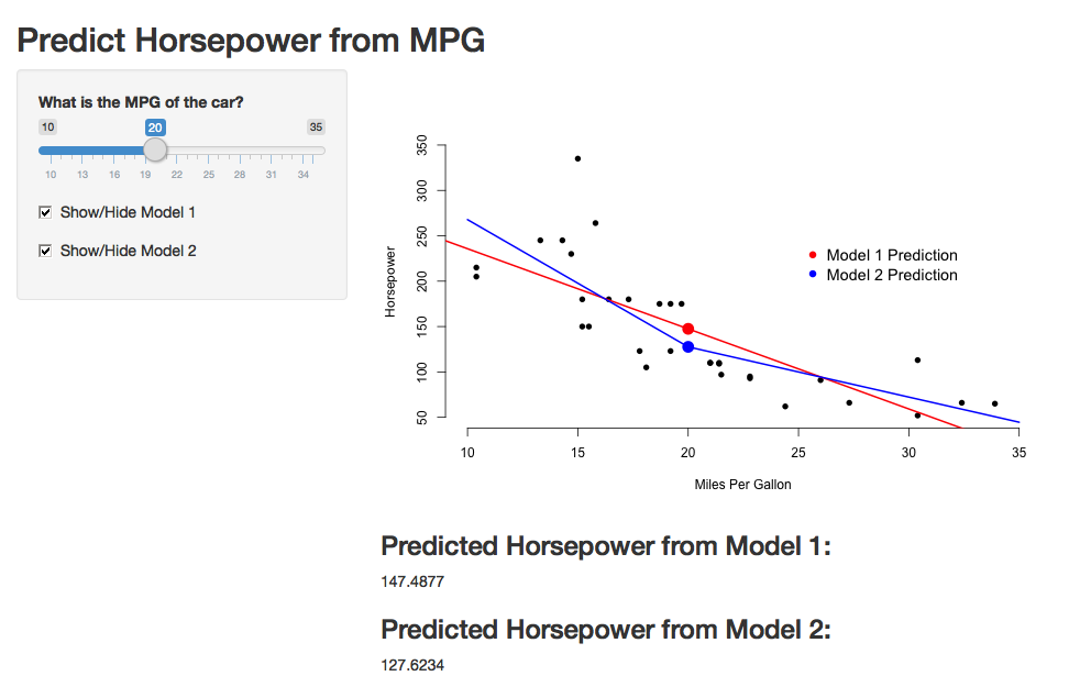
Modeling Cars

Make sure to runs this app locally:

shiny::runGitHub("seankross/developing-data-products", subdir = "assets/shinyapps/app6/")

App 7: ui.R

library(shiny)

fluidPage(
  titlePanel("Predict Horsepower from MPG"),
  
  sidebarLayout(
    sidebarPanel(
      sliderInput("sliderMPG", "What is the MPG of the car?", 10, 35, value = 20),
      checkboxInput("showModel1", "Show/Hide Model 1", value = TRUE),
      checkboxInput("showModel2", "Show/Hide Model 2", value = TRUE),
      submitButton("Submit")
    ),
    
    mainPanel(
      plotOutput("plot1"),
      h3("Predicted Horsepower from Model 1:"),
      textOutput("pred1"),
      h3("Predicted Horsepower from Model 2:"),
      textOutput("pred2")
    )
  )
)

The code above will produce an app that looks like this:

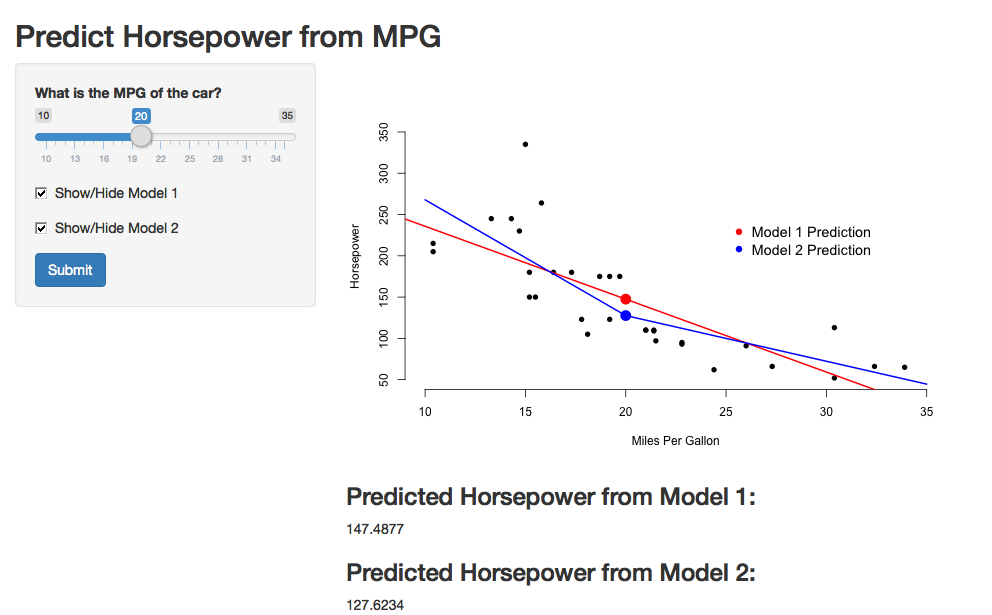
Delayed Computation

You can run this app locally like so:

shiny::runGitHub("seankross/developing-data-products", subdir = "assets/shinyapps/app7/")

2.7 Interactivity

App 8: ui.R

library(shiny)

fluidPage(
  titlePanel("Brush Points to Visualize Model"),
  sidebarLayout(
    sidebarPanel(
      h3("Slope"),
      textOutput("slopeOut"),
      h3("Intercept"),
      textOutput("intOut")
    ),
    mainPanel(
      plotOutput("plot1", brush = brushOpts(
        id = "brush1"
      ))
    )
  )
)

App 8: server.R

library(shiny)

function(input, output) {
  model <- reactive({
    brushed_data <- brushedPoints(trees, input$brush1,
                                  xvar = "Girth", yvar = "Volume")
    if(nrow(brushed_data) < 2){
      return(NULL)
    }
    lm(Volume ~ Girth, data = brushed_data)
  })
  
  output$slopeOut <- renderText({
    if(is.null(model())){
      "No Model Found"
    } else {
      model()[[1]][2]
    }
  })
  
  output$intOut <- renderText({
    if(is.null(model())){
      "No Model Found"
    } else {
      model()[[1]][1]
    }
  })
  
  output$plot1 <- renderPlot({
    plot(trees$Girth, trees$Volume, xlab = "Girth",
         ylab = "Volume", main = "Tree Measurements",
         cex = 1.5, pch = 16, bty = "n")
    if(!is.null(model())){
      abline(model(), col = "blue", lwd = 2)
    }
  })
}

The code above will produce an app that looks like this:

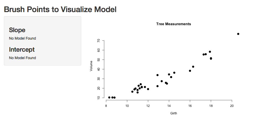
Brushed Points

You can run this app locally like so:

shiny::runGitHub("seankross/developing-data-products", subdir = "assets/shinyapps/app8/")

2.9 Conclusion

If you’re like most R users when you first encounter shiny, you’re probably wondering “What is going on? Why is the syntaxt so strange?” To get used to programming shiny apps, you need to throw away a little of your thinking about R; it’s a different style of programming.

Let’s parse through what’s going on with our two files to hopefully make things more clear. The ui.R function is controlling the interface. The function shinyUI is alerting R to that. The interior function, fluidPage is telling shinyUI what kind of page to create. In this case, it’s a page that can rearrange itself based on what you include in the UI, and it can rearrange itself so the app is easy to use on mobile screens. You specify all elements of the page using functions. In this case we want a title titlePanel("Data science FTW!"). Then we want the sidebarPanel to contain certain elements. So, the sidebarPanel function then takes arguments (again functions) of its elements. The statement h3('Sidebar text') is saying that we want the text Siderbar text in the sidebar (since this function occurs within the function sidebarPanel) and we want it to be at the font size h3. If you know a little html, you’ll recognize h3 as the third heading level font size. Similar to the sidebarPanel function, the mainPanel function takes functional arguments for the main panel.

Probably the most frequent syntaxt error for shiny is not putting commas in the right places of ui.R. Remember, the page elements are input as arguments, so they need commas like all arguments to R functions.arguments

The server.R file is a little easier. The function shinyServer tells R that it’s dealing with a shiny server. The server function always take an argument of an anonymous function with arguments inputs and outputs. In this case, our function doesn’t do anything.

2.10 Style and markup

Perhaps the easiest way to illustrate markup is through an example. While keeping the server.R file the same, change the ui.R file to the following:

{lang=r,line-numbers=off} _~ shinyUI(pageWithSidebar( headerPanel(“Illustrating markup”), sidebarPanel( h1(‘Sidebar panel’), h1(‘H1 text’), h2(‘H2 Text’), h3(‘H3 Text’), h4(‘H4 Text’)

), mainPanel( h3(‘Main Panel text’), code(‘some code’), p(‘some ordinary text’) ) )) _~

This produces the output:

Markup from shiny.

2.11 Different input types

Shiny allows for many different input types. In the following example, we change ui.R to allow for a few different input types. After you get the hang of these, any new ones will be easy. We leave server.R as is, so our inputs don’t do anything. See below the numeric input, checkbox, and date input.

{lang=r,line-numbers=off} _~ shinyUI(pageWithSidebar( headerPanel(“Illustrating inputs”), sidebarPanel( numericInput(‘id1’, ‘Numeric input, labeled id1’, 0, min = 0, max = 10, step = 1), checkboxGroupInput(“id2”, “Checkbox”, c(“Value 1” = “1”, “Value 2” = “2”, “Value 3” = “3”)), dateInput(“date”, “Date:”)
), mainPanel(

) )) _~

Run this to see the inputs. They’re also shown in the next image a few paragraphs below.

Refer to this lesson on the shiny tutorial site for a complete list of inputs available. Once you get the hang of one or two of them, then the remainder will be easy. So, do the above example first and then move on to trying some of the others.

Right now, nothing is done with our inputs. Let’s see if we can figure output how to at least get them into server.R.

2.12 Making your site interactive

Now that we have a bit of a handle on creating a shiny user interface, let’s make server.R reactive to the inputs from ui.R. First, let’s adapt our previous simple ui.R file to illustrate. Take the last example, where we collected a numeric input, checkbox and a date, and replace the mainPanel function with below.

{lang=r,line-numbers=off} _{_{_{mainPanel( h3(‘Illustrating outputs’), h4(‘You entered’), verbatimTextOutput(“oid1”), h4(‘You entered’), verbatimTextOutput(“oid2”), h4(‘You entered’), verbatimTextOutput(“odate”) )}}}

Our goal is to have our sidebarPanel collect the inputs and our main panel display them. The variables oid1, oid2 and odate are all outcome variables that we define in our server.R function. Here it is:

{lang=r,line-numbers=off} _~ shinyServer( function(input, output) { output$oid1 = renderPrint({input$id1}) output$oid2 = renderPrint({input$id2}) output$odate = renderPrint({input$date}) } ) _~

So, our function takes in input$id1 and prints out oid1. Note that id1 was the name given to our numeric input in our ui.R function. This is storred in input$id1. The label id2 was given to our checkbox data in ui.R and it’s value is storred in input$id2. Similarly, date was the label given to the input date and it is stored in input$date.

It is important in server.R to break from how we think about R programs being executed linearly. Instead, think of the functions being executed reactively to changing input from the ui.R function. The renderPrint function take the reactive input and assigns it to the output variable. Note the peculiar syntax for renderPrint in the ({R Statements }).

In this case, our server.R function is merely taking our inputed data and returning it right back. We named our output variables oid1, oid2 and odate, the same names used in ui.R. The renderPrint statement says that it is being sent back to ui.R for formatted display.

Here’s an example of the running of the code:

Example of input/output in Shiny.

2.13 Putting it all together

Now let’s build our prediction algorithm. For the ui.R files, let’s try

{lang=r,line-numbers=off} _~ shinyUI( pageWithSidebar( # Application title headerPanel(“Diabetes prediction”),

sidebarPanel(
  numericInput('glucose', 'Glucose mg/dl', 90, min = 50, max = 200, step = 5),
  submitButton('Submit')
),
mainPanel(
    h3('Results of prediction'),
    h4('You entered'),
    verbatimTextOutput("inputValue"),
    h4('Which resulted in a prediction of '),
    verbatimTextOutput("prediction")
)

) ) _~ So, we have a sidebar panel that takes in the glucose value. The submitButton puts a button that waits until the button is pressed to send values to sever.R. We’ll discuss more on submit buttons in the next chapter. The main panel shows the output. Notice that verbatimTextOutput is the function that is used to display the output of our server.R functions.

Our server.R function is

{lang=r,line-numbers=off} _~ diabetesRisk <- function(glucose) glucose / 200

shinyServer( function(input, output) { output$inputValue <- renderPrint({input$glucose}) output$prediction <- renderPrint({diabetesRisk(input$glucose)}) } ) _~ Notice that our prediction function is defined outside of the shinyServer function. The shinyServer function takes in the input and repeats both the input glucose level and the outputted diabetes risk.

The output of the function is show below

Output of our diabetes risk assessment score.

2.14 Another example

A great way to use shiny is to create interactive graphics. Let’s go through a simple example exactly like the one we did in the manipulate chapter. The benifit of using shiny over manipulate is the ability to share the app broadly as a web page.

Here’s our ui.R function

{lang=r,line-numbers=off} _~ shinyUI(pageWithSidebar( headerPanel(“Example plot”), sidebarPanel( sliderInput(‘mu’, ‘Guess at the mean’,value = 70, min = 62, max = 74, step = 0.05,) ), mainPanel( plotOutput(‘newHist’) ) )) _~

Notice that plotOutput is the function used for plotting our generated histogram. Let’s consider the server.R function.

{lang=r,line-numbers=off} _~ library(UsingR) data(galton)

shinyServer( function(input, output) { output$newHist <- renderPlot({ hist(galton$child, xlab=‘child height’, col=‘lightblue’,main=‘Histogram’) mu <- input$mu lines(c(mu, mu), c(0, 200),col="red",lwd=5) mse <- mean((galton$child - mu)^2) text(63, 150, paste(“mu =”, mu)) text(63, 140, paste(“MSE =”, round(mse, 2))) }) } ) _~

This shows how we created a somewhat elaborate set of code in the renderPlot statement that generates the plot. Specifically note the line mu <- input$mu. This is our slider value that we use to generate our horizontal line. The final output is shown below:

Output of our interactive plotting example.

2.15 Sharing your app

Now that we have a working app we’d like to share it with the world. You could simply post the code, and whatever data files are needed, then users could use runApp to see the application. However, it’s much nicer to have it display as a stand alone web application. This requires running a shiny server to host the app. Instead of creating and deploying our own shiny server, we’ll rely on RStudio’s service shinyapps.io. You can go to https://www.shinyapps.io/ where you will be shown how to create an account. After creating the account, you’ll be able to host your shiny apps there. Note, this is a freemium service, so that if you want to host a lot of apps, and have fancy bells and whistles, you’ll have to spring for the paid service (or host your own shiny server).

After getting a login, you’ll have to do some basic installs. First, devtools. (This is an essential package for a variety of reasons.) So, do install.packages("devtools") at the R command prompt. This will allow you to install the shinyapps package directly from github with the command devtools::install_github('rstudio/shinyapps').

Next you have to run some code that you can copy from the shinyapps.io site. It looks like

{lang=r,line-numbers=off} _{_{_{shinyapps::setAccountInfo(name=‘’, token=‘’, secret=‘’)}}}

This tells RStudio how to submit your code to shinyapps.io and gives it the permissions to do so. Now, change to the directory where your server.R and ui.R files are at and you can submit your code with:

{lang=r,line-numbers=off} _~ deployApp(appName = “myFirstApp”) _~

Make sure that shinyapps is loaded (with library(shinyapps)). If you need a path to your files, put that in the argument to deployApp. The appName argument appears to be necessary, and you want it anyway so you know which app it is on shinyapps.io. If all has gone well, your app will launch and it will open up a browser window linking to it. In my case, the link was. https://bcaffo.shinyapps.io/myFirstApp.

You can manage your app in the browswer at shinyapps.io. Now when you go to shinyapps.io and click on Applications/All, or Applicatons/Running then you should see your app.

Example app listing at shinyapps.io

From here you can start, stop and delete your app. You can also do that in your R console, with the shinapps tools. I would recommend using the web browswer as it’s a little easier, but if you get to the point where you’re writing a lot of apps, you probably want to learn the console commands.

2.16 talk about shiny server later

It is important to dinstiguish between a Shiny applications (app) and a Shiny server. A Shiny server is required to host a shiny app for the world. Otherwise, only those who have have shiny installed and have access to your code could run your web application, which in some cases defeats the purpose of making a web application in the first place. In this book, we won’t cover creating a shiny server, as that requires understanding a little linux server administration. Instead, we’ll run our apps locally and use RStudio’s service for hosting shiny apps (their servers) on a platform called shinyapps.io.

RStudio does the server work for your so that all you need to worry about is building your app. Shinyapps.io is free up to a point in that you can only run 5 apps for a certain amount of time per month. This will be fine for our purposes, but if you’re really going to get into making Shiny apps, you’ll have to spring for a paid plan or run your own server.

Chapter 2 Shiny

2.1 Installing Shiny

2.2 Your First Shiny App

2.3 More UI Elements

2.4 Inputs and Outputs

2.5 Dynamic UI

2.6 Reactivity

2.7 Interactivity

2.8 Sharing Apps

2.9 Conclusion

2.10 Style and markup

2.11 Different input types

2.12 Making your site interactive

2.13 Putting it all together

2.14 Another example

2.15 Sharing your app

2.16 talk about shiny server later