OK, statistics friends, point me to a good explanation of the wrong/right interpretations of confidence intervals?
— Julia Silge (@juliasilge) May 4, 2016
Imagine you’re trying to estimate a statistic like the mean of a population. First let’s make a population of Gaussian random variables.
set.seed(2016-05-04)
population <- rnorm(100000)
We’re trying to estimate the true mean of this population which is 0.0031898.
Normally we can’t measure every member of this population, so we have to sample the population. Let’s take a sample.
first_sample <- sample(population, 100)
Now we’ll construct a 95% confidence interval for the mean of this population:
# Lower bound
lb <- mean(first_sample) - 1.96 * (sd(first_sample)/sqrt(length(first_sample)))
lb

## [1] -0.1360584

# Upper bound
ub <- mean(first_sample) + 1.96 * (sd(first_sample)/sqrt(length(first_sample)))
ub

## [1] 0.2337529
So what does this confidence interval really mean? If we take samples from this population many many times, the true mean of the population will be contained within each sample confidence interval 95% of the time. Let’s test this theory:
# Each column of `samples` is a sample of size 100 from the
# population. We're taking 10000 samples.
samples <- replicate(10000, sample(population, 100))

lower_bounds <- apply(samples, 2, function(row){
  mean(row) - 1.96 * (sd(row)/sqrt(length(row)))
})
upper_bounds <- apply(samples, 2, function(row){
  mean(row) + 1.96 * (sd(row)/sqrt(length(row)))
})

true_mean <- mean(population)

# This is just a way of saying: how many confidence
# intervals contain the true mean?
mean(true_mean > lower_bounds & true_mean < upper_bounds)

## [1] 0.9489
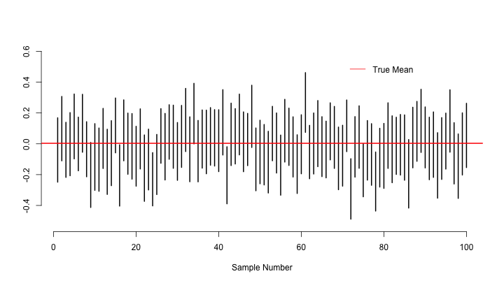
Visualizing these confidence intervals in the style of Hadley Wickham’s notes:
# Only considering the first 100 confidence intervals
plot(0, 0, xlim = c(1, 100), ylim = c(min(lower_bounds), max(upper_bounds)),
     xlab = "Sample Number", ylab = "", bty = "n", col = "white")
for(i in 1:100){
  segments(i, lower_bounds[i], i, upper_bounds[i], lwd = 2)
}
abline(h = true_mean, col = "red", lwd = 2)
legend(70, .55, legend = "True Mean", col = "red", lty = 1, bty = "n")