A Sentiment Analysis of Hamilton

The broom Where it Happens / When are these #rcatladies gonna rise up?

I was raised listening to musicals and I’ve occasionally performed in a few, so naturally over the past year I’ve been listening to Hamilton on repeat to the point where the image of a five pointed star is burned into my iPhone screen. I’ve also been wanting to take the tidytext R package for a spin after seeing what creators Julia Silge and David Robinson have been able to do with it, not to mention that The Economist uses it!

Hamilton is a particularly good musical to analyze because the show is sung-through, meaning that the entirety of the plot is contained in the lyrics. We can get the lyrics by scraping a lyrics website with rvest. Let’s start by scraping a list of web pages that contain the lyrics for each song:

library(rvest)
library(magrittr)

ham_raw <- read_html("http://www.allmusicals.com/h/hamilton.htm")

ham_lyrics_pages <- ham_raw %>%
  html_nodes(".lyrics-list") %>%
  html_nodes("a") %>%
  html_attr("href")

head(ham_lyrics_pages)

## [1] "http://www.allmusicals.com/lyrics/hamilton/alexanderhamilton.htm" 
## [2] "http://www.allmusicals.com/lyrics/hamilton/aaronburrsir.htm"      
## [3] "http://www.allmusicals.com/lyrics/hamilton/myshot.htm"            
## [4] "http://www.allmusicals.com/lyrics/hamilton/thestoryoftonight.htm" 
## [5] "http://www.allmusicals.com/lyrics/hamilton/theschuylersisters.htm"
## [6] "http://www.allmusicals.com/lyrics/hamilton/farmerrefuted.htm"

Now I can scrape each individual page for the lyrics:

library(stringr)

# Pre-allocating a list
ham_song_lyrics <- vector(mode = "list", length = length(ham_lyrics_pages))

for (i in seq_along(ham_song_lyrics)) {
  lyrics_raw <- read_html(ham_lyrics_pages[i])
  ham_song_lyrics[[i]] <- lyrics_raw %>%
    html_nodes("div#page") %>%
    html_text() %>%
    strsplit("\r\n") %>%
    unlist()
  song_name <- str_extract(ham_lyrics_pages[i], "[a-z|0-9]+\\.htm") %>%
    str_replace("\\.htm", "")
  names(ham_song_lyrics[[i]]) <- rep(song_name, length(ham_song_lyrics[[i]]))
}

ham_song_lyrics %<>% unlist()

# Some data cleaning

library(
  # Pardon me, are you Aaron
  purrr
  # sir?
  )

ham_song_lyrics %<>%
  map_chr(gsub, pattern = "Last Update.+", replacement = "") %>%
  discard(function(x) grepl("\\[|\\]", x)) %>%
  discard(function(x) c("^Hamilton:$", "^Eliza:$", "^Angelica:$",
                        "^Lafayette:$", "^Choirs:$", "Chorus:$",
                        "^Both:$", "^Mulligan:$", "^Laurens:$", 
                        "^King George:$") %>%
                        map_lgl(grepl, x = x) %>% any())

# Making a Tidy Data Frame of lyrics

library(dplyr)

ham_lyric_tbl <- data.frame(lyric = ham_song_lyrics,
                            song = names(ham_song_lyrics),
                            stringsAsFactors = FALSE) %>%
  mutate(line = row_number())

library(knitr)
kable(ham_lyric_tbl[896:900,1:2], format = "html", 
      row.names=FALSE)

lyric	song
So so so so this is what it feels like to match wits with someone at your level.	satisfied
What the hell is the catch?	satisfied
It's the feeling of freedom of seeing the light.	satisfied
It's Ben Franklin with the key and the kite.	satisfied
You see it right?	satisfied

Okay we’ve got the lyrics in a data frame! Now we can tidy this data frame even further so that each “token” (essentially each word) is ready for sentiment analysis.

library(tidytext)

ham_token_tbl <- ham_lyric_tbl %>%
  unnest_tokens(word, lyric) %>%
  anti_join(stop_words)

Now that each song is tokenized we can start exploring the data. Let’s take a look at the most common words in the show:

ham_token_tbl %>%
  count(word, sort = TRUE) %>%
  slice(1:15) %>%
  kable(format = "html", row.names=FALSE)

word	n
i’m	160
da	109
hamilton	87
time	85
wait	78
don’t	70
burr	69
you’re	68
shot	58
sir	56
hey	52
alexander	51
it’s	48
rise	41
whoa	40

I like how this forms a little song of its own: “I’m da Hamilton! Time? Wait! Don’t Burr, you’re shot sir! Hey Alexander!” Next let’s examine which pairs of words appear together most often in a verse:

ham_grams <- ham_token_tbl %>%
  pair_count(line, word, sort = TRUE)

ham_grams %>%
  slice(1:10) %>%
  kable(format = "html", row.names=FALSE, align = "c")

value1	value2	n
throwing	shot	24
hamilton	alexander	21
president	gon	18
running	time	17
president	he’s	14
stay	alive	13
neuf	huit	12
huit	sept	12
gon	he’s	12
em	i’m	12

“Alexander” and “Hamilton” are no surprise, but we can also see how the songs “My Shot,” “Non-Stop,” and “The Reynolds Pamphlet” dominate these common word pairings. We can visualize words that commonly appear with other words across different verses as a network:

library(igraph)
library(ggraph)

set.seed(1776) # New York City
ham_grams %>%
        filter(n >= 5) %>%
        graph_from_data_frame() %>%
        ggraph(layout = "fr") +
        geom_edge_link(aes(edge_alpha = n, edge_width = n)) +
        geom_node_point(color = "#0052A5", size = 5) +
        geom_node_text(aes(label = name), vjust = 1.5) +
        ggtitle(expression(paste("Word Network in Lin-Manuel Miranda's ", 
                                 italic("Hamilton")))) +
        theme_void()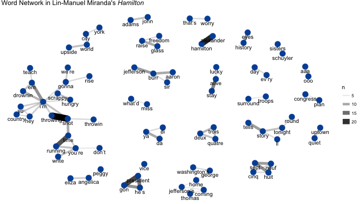

It’s interesting to see how many of the major lyrical themes can be seen in this network, including how “shot <-> throwing” is related to “time <-> running.” Also notice how the theme of “coming/going home” links George Washington and Thomas Jefferson.

Now let’s perform the sentiment analysis. Sentiment spans a positive/negative axis, which we’ll map over the course of the show. We’ll evaluate sentiment on a song-by-song basis. A LOESS smoothing line is a good way to track the general sentiment of the show:

# Creating the set of sentiments we'll use
nrc <- sentiments %>%
  filter(lexicon == "nrc") %>%
  select(-score, -lexicon) %>%
  filter(sentiment %in% c("positive", "negative"))

# Joining sentiment and song
library(tidyr)
hamilton_sentiment <- ham_token_tbl %>%
  inner_join(nrc) %>% 
  count(index = song, sentiment) %>% 
  spread(sentiment, n, fill = 0) %>% 
  mutate(sentiment = positive - negative)

# Putting the songs back in order
ham_song_names_tbl <- data.frame(num = 1:length(ham_lyrics_pages))
ham_song_names_tbl$index <- str_extract(ham_lyrics_pages, "[a-z|0-9]+\\.htm") %>%
  str_replace("\\.htm", "")

hamilton_sentiment %<>%
  left_join(ham_song_names_tbl) %>%
  arrange(num)

plot(hamilton_sentiment$sentiment, bty = "n",
     xlab = "Song Number", ylab = "Sentiment",
     main = "Sentiment Analysis of Hamilton",
     pch = 19, col = "#E0162B")

loess_ham <- loess.smooth(hamilton_sentiment$num,
                          hamilton_sentiment$sentiment,
                          span = .15, degree = 2)

lines(loess_ham, col = "#0052A5", lwd = 5)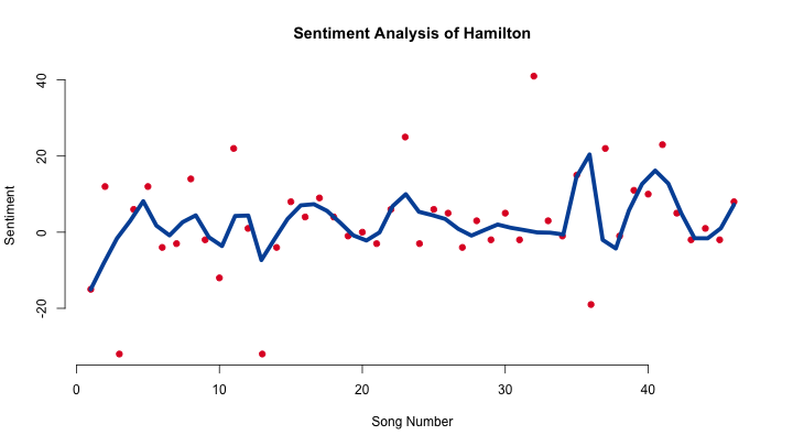

The first three peaks show the first major positive events in Hamilton’s life: meeting his friends, becoming Washington’s secretary, and then meeting and marrying Eliza. The fourth peek around the 15th song encompasses the events of the Revolutionary War, and the peak after the 20th song occurs at the same time as the song “Non-Stop,” one of the most energetic songs in the show. Around the 35th song there’s a big peak which is influenced by the fact that “One Last Time” is given a very high sentiment rating, but that peak quickly falls off with “Hurricane” which is the 36th song. The last peak shows Hamilton and and Eliza rebuilding their relationship, peaking with “It’s Quiet Uptown,” with the show then descending into the Hamilton-Burr duel.

Closing Thoughts

Text and sentiment analysis seem to capture several of the major themes and movements in Hamilton’s plot, but under close examination some of the sentiment scores of certain songs don’t make sense in the context of the show. For example: although I think of “My Shot” as a positive song it has a sentiment score of -32, meanwhile “One Last Time” which is more melancholy has a score of 41. It would be interesting to get musical theater scholars and a computational sentiment experts to work together to “validate” particular sentiment values and techniques against a consensus of literary/theatrical meaning. It would also be very interesting to analyze the sentiment of the music in every song and to see how that correlates with the sentiment of the words.

Thank you again to Julia Silge and David Robinson for building these tools and for providing fantastic examples for their use.

library(rvest)
library(magrittr)

ham_raw <- read_html("http://www.allmusicals.com/h/hamilton.htm")

ham_lyrics_pages <- ham_raw %>%
  html_nodes(".lyrics-list") %>%
  html_nodes("a") %>%
  html_attr("href")

head(ham_lyrics_pages)

## [1] "http://www.allmusicals.com/lyrics/hamilton/alexanderhamilton.htm" 
## [2] "http://www.allmusicals.com/lyrics/hamilton/aaronburrsir.htm"      
## [3] "http://www.allmusicals.com/lyrics/hamilton/myshot.htm"            
## [4] "http://www.allmusicals.com/lyrics/hamilton/thestoryoftonight.htm" 
## [5] "http://www.allmusicals.com/lyrics/hamilton/theschuylersisters.htm"
## [6] "http://www.allmusicals.com/lyrics/hamilton/farmerrefuted.htm"

Now I can scrape each individual page for the lyrics:

library(stringr)

# Pre-allocating a list
ham_song_lyrics <- vector(mode = "list", length = length(ham_lyrics_pages))

for (i in seq_along(ham_song_lyrics)) {
  lyrics_raw <- read_html(ham_lyrics_pages[i])
  ham_song_lyrics[[i]] <- lyrics_raw %>%
    html_nodes("div#page") %>%
    html_text() %>%
    strsplit("\r\n") %>%
    unlist()
  song_name <- str_extract(ham_lyrics_pages[i], "[a-z|0-9]+\\.htm") %>%
    str_replace("\\.htm", "")
  names(ham_song_lyrics[[i]]) <- rep(song_name, length(ham_song_lyrics[[i]]))
}

ham_song_lyrics %<>% unlist()

# Some data cleaning

library(
  # Pardon me, are you Aaron
  purrr
  # sir?
  )

ham_song_lyrics %<>%
  map_chr(gsub, pattern = "Last Update.+", replacement = "") %>%
  discard(function(x) grepl("\\[|\\]", x)) %>%
  discard(function(x) c("^Hamilton:$", "^Eliza:$", "^Angelica:$",
                        "^Lafayette:$", "^Choirs:$", "Chorus:$",
                        "^Both:$", "^Mulligan:$", "^Laurens:$", 
                        "^King George:$") %>%
                        map_lgl(grepl, x = x) %>% any())

# Making a Tidy Data Frame of lyrics

library(dplyr)

ham_lyric_tbl <- data.frame(lyric = ham_song_lyrics,
                            song = names(ham_song_lyrics),
                            stringsAsFactors = FALSE) %>%
  mutate(line = row_number())

library(knitr)
kable(ham_lyric_tbl[896:900,1:2], format = "html", 
      row.names=FALSE)

lyric	song
So so so so this is what it feels like to match wits with someone at your level.	satisfied
What the hell is the catch?	satisfied
It's the feeling of freedom of seeing the light.	satisfied
It's Ben Franklin with the key and the kite.	satisfied
You see it right?	satisfied

Okay we’ve got the lyrics in a data frame! Now we can tidy this data frame even further so that each “token” (essentially each word) is ready for sentiment analysis.

library(tidytext)

ham_token_tbl <- ham_lyric_tbl %>%
  unnest_tokens(word, lyric) %>%
  anti_join(stop_words)

Now that each song is tokenized we can start exploring the data. Let’s take a look at the most common words in the show:

ham_token_tbl %>%
  count(word, sort = TRUE) %>%
  slice(1:15) %>%
  kable(format = "html", row.names=FALSE)

word	n
i’m	160
da	109
hamilton	87
time	85
wait	78
don’t	70
burr	69
you’re	68
shot	58
sir	56
hey	52
alexander	51
it’s	48
rise	41
whoa	40

ham_grams <- ham_token_tbl %>%
  pair_count(line, word, sort = TRUE)

ham_grams %>%
  slice(1:10) %>%
  kable(format = "html", row.names=FALSE, align = "c")

value1	value2	n
throwing	shot	24
hamilton	alexander	21
president	gon	18
running	time	17
president	he’s	14
stay	alive	13
neuf	huit	12
huit	sept	12
gon	he’s	12
em	i’m	12

library(igraph)
library(ggraph)

set.seed(1776) # New York City
ham_grams %>%
        filter(n >= 5) %>%
        graph_from_data_frame() %>%
        ggraph(layout = "fr") +
        geom_edge_link(aes(edge_alpha = n, edge_width = n)) +
        geom_node_point(color = "#0052A5", size = 5) +
        geom_node_text(aes(label = name), vjust = 1.5) +
        ggtitle(expression(paste("Word Network in Lin-Manuel Miranda's ", 
                                 italic("Hamilton")))) +
        theme_void()

# Creating the set of sentiments we'll use
nrc <- sentiments %>%
  filter(lexicon == "nrc") %>%
  select(-score, -lexicon) %>%
  filter(sentiment %in% c("positive", "negative"))

# Joining sentiment and song
library(tidyr)
hamilton_sentiment <- ham_token_tbl %>%
  inner_join(nrc) %>% 
  count(index = song, sentiment) %>% 
  spread(sentiment, n, fill = 0) %>% 
  mutate(sentiment = positive - negative)

# Putting the songs back in order
ham_song_names_tbl <- data.frame(num = 1:length(ham_lyrics_pages))
ham_song_names_tbl$index <- str_extract(ham_lyrics_pages, "[a-z|0-9]+\\.htm") %>%
  str_replace("\\.htm", "")

hamilton_sentiment %<>%
  left_join(ham_song_names_tbl) %>%
  arrange(num)

plot(hamilton_sentiment$sentiment, bty = "n",
     xlab = "Song Number", ylab = "Sentiment",
     main = "Sentiment Analysis of Hamilton",
     pch = 19, col = "#E0162B")

loess_ham <- loess.smooth(hamilton_sentiment$num,
                          hamilton_sentiment$sentiment,
                          span = .15, degree = 2)

lines(loess_ham, col = "#0052A5", lwd = 5)

Closing Thoughts

Thank you again to Julia Silge and David Robinson for building these tools and for providing fantastic examples for their use.