My brother and I were talking about saving for retirement, specifically whether he should wait to invest in his IRA until he gets a large stipend at the end of the summer or if he should invest a smaller amount of money (~$100 per week) throughout the year. Some people call the first approach “lump sum investing” and the latter appraoch “dollar cost averaging.” This post is an attempt to visualize the difference between these two approaches.
We’re both customers of Charles Schwab which allows us to buy their funds without paying a commission. Their broad US stock market ETF is called SCHB. Let’s get SCHB’s opening price for the last year.
set.seed(2016-06-15)
options(digits = 2)

# Get SCHB data
library(quantmod)
schb <- getSymbols("SCHB", auto.assign = FALSE, from = "2015-06-15", to = "2016-06-15")
schb <- as.data.frame(schb)[,1]
Imagine that you bought 100 shares when the market openned on one of the days in the past year. Now imagine there are multiple universes where in each universe you bought all 100 shares of the ETF on a different day. Let’s see how much money you would have made/lost after a year in each universe:
# The cost of 100 shares on each trading day last year
starting_portfolio_values <- schb * 100
# The value of each "portfolio" after a year
last_day_portfolio_value <- starting_portfolio_values[length(schb)]

hist(last_day_portfolio_value - starting_portfolio_values,
     main = "Histogram of Change in Value",
     xlab = "Change in Value", breaks = 15,
     col = rgb(1, 0, 0, .6))
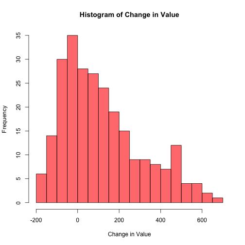
On average you would have made $118.91, but you can see that the range of outcomes is large: from $-174 to $667!
Now imagine that instead you bought 2 shares on 50 different random days last year. And to be fair this happened in the same number of universes as in the last example.
n_universes <- length(schb)
change_in_value <- replicate(n_universes, {
  # Pick 50 random days and buy 2 shares each day
  share_prices <- sample(schb, 50) * 2
  # Sum of the prices is the cost basis
  cost_basis <- sum(share_prices)
  # Compute the change in portfolio value
  last_day_portfolio_value - cost_basis
})

hist(change_in_value, breaks = 15, main = "Histogram of Change in Value",
     xlab = "Change in Value", col = rgb(0, 0, 1, .6))
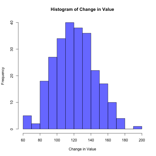
On average you would have made $121.19, and the range of outcomes is much smaller: from $63.86 to $195.78. In order to better compare these investment strategies I’ll plot both sets of outcomes on the same axis:
h1 <- hist(last_day_portfolio_value - starting_portfolio_values, breaks = 15)
h2 <- hist(change_in_value, breaks = 15)


hist_xmin <- min(last_day_portfolio_value - starting_portfolio_values)
hist_xmax <- max(last_day_portfolio_value - starting_portfolio_values)

plot(h1, col = rgb(1, 0, 0, .6), main = "Histogram of Change in Value",
     xlab = "Change in Value", xlim = c(hist_xmin, hist_xmax), ylim = c(0, 40))
plot(h2, col = rgb(0, 0, 1, .6), main = "Histogram of Change in Value",
     xlab = "Change in Value", add = TRUE)
legend(350, 30, c("Lump Sum Investing", "Dollar Cost Averaging"), pch = rep(15, 2),
       col = c(rgb(1, 0, 0, .6), rgb(0, 0, 1, .6)), bty = "n", cex = 1.5)
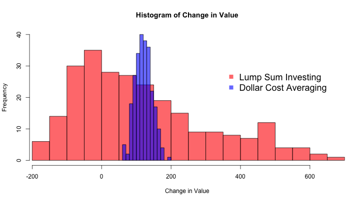
There are many generalizations in this analysis (there are no commissions, only one kind of investment is considered, etc) however you can see that investing small sums of money over time seems to restrict the range of your gains and losses around a mean value that is close the average gains and losses you would have if you invested a large amount of money all at once.